{
	"active_requests": {
	  "clientContextID": "805f519d-0ffb-4adf-bd19-15238c95900a",
	  "elapsedTime": "645.4333ms",
	  "executionTime": "645.4333ms",
	  "node": "10.0.75.1",
	  "phaseCounts": {
		"fetch": 6672,
		"primaryScan": 7171
	  },
	  "phaseOperators": {
		"fetch": 1,
		"primaryScan": 1
	  },
	  "phaseTimes": {
		"authorize": "500.3µs",
		"fetch": "365.7758ms",
		"parse": "500µs",
		"primaryScan": "107.3891ms"
	  },
	  "requestId": "80787238-f4cb-4d2d-999f-7faff9b081e4",
	  "requestTime": "2017-02-10 09:06:18.3526802 -0500 EST",
	  "scanConsistency": "unbounded",
	  "state": "running",
	  "statement": "select * from `travel-sample`;"
	}
}New Profiling and Monitoring in Couchbase Server 5.0 Preview
This is a repost that originally appeared on the Couchbase Blog: New Profiling and Monitoring in Couchbase Server 5.0 Preview.
N1QL query monitoring and profiling updates are just some of goodness you can find in February’s developer preview release of Couchbase Server 5.0.0.
Go download the February 5.0.0 developer release of Couchbase Server today, click the "Developer" tab, and check it out. You still have time to give us some feedback before the official release.
As always, keep in mind that I’m writing this blog post on early builds, and some things may change in minor ways by the time you get the release.
What is profiling and monitoring for?
When I’m writing N1QL queries, I need to be able to understand how well (or how badly) my query (and my cluster) is performing in order to make improvements and diagnose issues.
With this latest developer version of Couchbase Server 5.0, some new tools have been added to your N1QL-writing toolbox.
N1QL Writing Review
First, some review.
There are multiple ways for a developer to execute N1QL queries.
-
Use the SDK of your choice.
-
Use the cbq command line tool.
-
Use the Query Workbench in Couchbase Web Console
-
Use the REST API N1QL endpoints
In this post, I’ll be mainly using Query Workbench.
There are two system catalogs that are already available to you in Couchbase Server 4.5 that I’ll be talking about today.
-
system:active_request - This catalog lists all the currently executing active requests or queries. You can execute the N1QL query
SELECT * FROM system:active_requests;and it will list all those results. -
system:completed_requests - This catalog lists all the recent completed requests (that have run longer than some threshold of time, default of 1 second). You can execute
SELECT * FROM system:completed_requests;and it will list these queries.
New to N1QL: META().plan
Both active_requests and completed_requests return not only the original N1QL query text, but also related information: request time, request id, execution time, scan consistency, and so on. This can be useful information. Here’s an example that looks at a simple query (select * from `travel-sample`) while it’s running by executing select * from system:active_requests;
First, I want to point out that phaseTimes is a new addition to the results. It’s a quick and dirty way to get a sense of the query cost without looking at the whole profile. It gives you the overall cost of each request phase without going into detail of each operator. In the above example, for instance, you can see that parse took 500µs and primaryScan took 107.3891ms. This might be enough information for you to go on without diving into META().plan.
However, with the new META().plan, you can get very detailed information about the query plan. This time, I’ll execute SELECT *, META().plan FROM system:active_requests;
[
  {
    "active_requests": {
      "clientContextID": "75f0f401-6e87-48ae-bca8-d7f39a6d029f",
      "elapsedTime": "1.4232754s",
      "executionTime": "1.4232754s",
      "node": "10.0.75.1",
      "phaseCounts": {
        "fetch": 12816,
        "primaryScan": 13231
      },
      "phaseOperators": {
        "fetch": 1,
        "primaryScan": 1
      },
      "phaseTimes": {
        "authorize": "998.7µs",
        "fetch": "620.704ms",
        "primaryScan": "48.0042ms"
      },
      "requestId": "42f50724-6893-479a-bac0-98ebb1595380",
      "requestTime": "2017-02-15 14:44:23.8560282 -0500 EST",
      "scanConsistency": "unbounded",
      "state": "running",
      "statement": "select * from `travel-sample`;"
    },
    "plan": {
      "#operator": "Sequence",
      "#stats": {
        "#phaseSwitches": 1,
        "kernTime": "1.4232754s",
        "state": "kernel"
      },
      "~children": [
        {
          "#operator": "Authorize",
          "#stats": {
            "#phaseSwitches": 3,
            "kernTime": "1.4222767s",
            "servTime": "998.7µs",
            "state": "kernel"
          },
          "privileges": {
            "default:travel-sample": 1
          },
          "~child": {
            "#operator": "Sequence",
            "#stats": {
              "#phaseSwitches": 1,
              "kernTime": "1.4222767s",
              "state": "kernel"
            },
            "~children": [
              {
                "#operator": "PrimaryScan",
                "#stats": {
                  "#itemsOut": 13329,
                  "#phaseSwitches": 53319,
                  "execTime": "26.0024ms",
                  "kernTime": "1.3742725s",
                  "servTime": "22.0018ms",
                  "state": "kernel"
                },
                "index": "def_primary",
                "keyspace": "travel-sample",
                "namespace": "default",
                "using": "gsi"
              },
              {
                "#operator": "Fetch",
                "#stats": {
                  "#itemsIn": 12817,
                  "#itemsOut": 12304,
                  "#phaseSwitches": 50293,
                  "execTime": "18.5117ms",
                  "kernTime": "787.9722ms",
                  "servTime": "615.7928ms",
                  "state": "services"
                },
                "keyspace": "travel-sample",
                "namespace": "default"
              },
              {
                "#operator": "Sequence",
                "#stats": {
                  "#phaseSwitches": 1,
                  "kernTime": "1.4222767s",
                  "state": "kernel"
                },
                "~children": [
                  {
                    "#operator": "InitialProject",
                    "#stats": {
                      "#itemsIn": 11849,
                      "#itemsOut": 11848,
                      "#phaseSwitches": 47395,
                      "execTime": "5.4964ms",
                      "kernTime": "1.4167803s",
                      "state": "kernel"
                    },
                    "result_terms": [
                      {
                        "expr": "self",
                        "star": true
                      }
                    ]
                  },
                  {
                    "#operator": "FinalProject",
                    "#stats": {
                      "#itemsIn": 11336,
                      "#itemsOut": 11335,
                      "#phaseSwitches": 45343,
                      "execTime": "6.5002ms",
                      "kernTime": "1.4157765s",
                      "state": "kernel"
                    }
                  }
                ]
              }
            ]
          }
        },
        {
          "#operator": "Stream",
          "#stats": {
            "#itemsIn": 10824,
            "#itemsOut": 10823,
            "#phaseSwitches": 21649,
            "kernTime": "1.4232754s",
            "state": "kernel"
          }
        }
      ]
    }
  }, ...
]
The above output comes from the Query Workbench.
Note the new "plan" part. It contains a tree of operators that combine to execute the N1QL query. The root operator is a Sequence, which itself has a collection of child operators like Authorize, PrimaryScan, Fetch, and possibly even more Sequences.
Enabling the profile feature
To get this information when using cbq or the REST API, you’ll need to turn on the "profile" feature.
You can do this in cbq by entering set -profile timings; and then running your query.
You can also do this with the REST API on a per request basis (using the /query/service endpoint and passing a querystring parameter of profile=timings, for instance).
You can turn on the setting for the entire node by making a POST request to http://localhost:8093/admin/settings, using Basic authentication, and a JSON body like:
{
  "completed-limit": 4000,
  "completed-threshold": 1000,
  "controls": false,
  "cpuprofile": "",
  "debug": false,
  "keep-alive-length": 16384,
  "loglevel": "INFO",
  "max-parallelism": 1,
  "memprofile": "",
  "pipeline-batch": 16,
  "pipeline-cap": 512,
  "pretty": true,
  "profile": "timings",
  "request-size-cap": 67108864,
  "scan-cap": 0,
  "servicers": 32,
  "timeout": 0
}
Notice the profile setting. It was previously set to off, but I set it to "timings".
You may not want to do that, especially on nodes being used by other people and programs, because it will affect other queries running on the node. It’s better to do this on a per-request basis.
It’s also what Query Workbench does by default.
Using the Query Workbench
There’s a lot of information in META().plan about how the plan is executed. Personally, I prefer to look at a simplified graphical version of it in Query Workbench by clicking the "Plan" icon (which I briefly mentioned in a previous post about the new Couchbase Web Console UI).
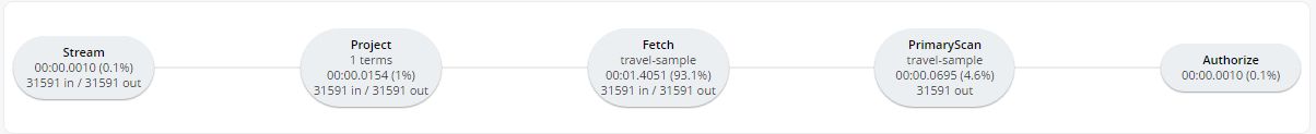
Let’s look at a slightly more complex example. For this exercise, I’m using the travel-sample bucket, but I have removed one of the indexes (DROP INDEX `travel-sample.def_sourceairport;`).
I then execute a N1QL query to find flights between San Francisco and Miami:
SELECT r.id, a.name, s.flight, s.utc, r.sourceairport, r.destinationairport, r.equipment
FROM `travel-sample` r
UNNEST r.schedule s
JOIN `travel-sample` a ON KEYS r.airlineid
WHERE r.sourceairport = 'SFO'
AND r.destinationairport = 'MIA'
AND s.day = 0
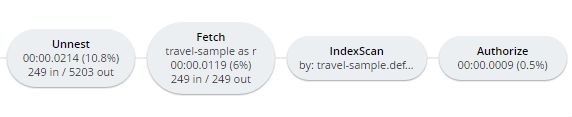
ORDER BY a.name;Executing this query (on my single-node local machine) takes about 10 seconds. That’s definitely not an acceptible amount of time, so let’s look at the plan to see what the problem might be (I broke it into two lines so the screenshots will fit in the blog post).
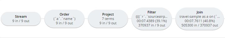
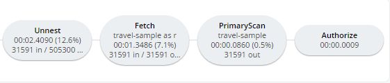
Looking at that plan, it seems like the costliest parts of the query are the Filter and the Join. JOIN operations work on keys, so they should normally be very quick. But it looks like there are a lot of documents being joined.
The Filter (the WHERE part of the query) is also taking a lot of time. It’s looking at the sourceairport and destinationairport fields. Looking elsewhere in the plan, I see that there is a PrimaryScan. This should be a red flag when you are trying to write performant queries. PrimaryScan means that the query couldn’t find an index other than the primary index. This is roughly the equivalent of a "table scan" in relational database terms. (You may want to drop the primary index so that these issues get bubbled-up faster, but that’s a topic for another time).
Let’s add an index on the sourceairport field and see if that helps.
CREATE INDEX `def_sourceairport` ON `travel-sample`(`sourceairport`);Now, running the same query as above, I get the following plan:
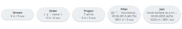
This query took ~100ms (on my single-node local machine) which is much more acceptible. The Filter and the Join still take up a large percentage of the time, but thanks to the IndexScan replacing the PrimaryScan, there are many fewer documents that those operators have to deal with. Perhaps the query could be improved even more with an additional index on the destinationairport field.
Beyond Tweaking Queries
The answer to performance problems is not always in tweaking queries. Sometimes you might need to add more nodes to your cluster to address the underlying problem.
Look at the PrimaryScan information in META().plan. Here’s a snippet:
"~children": [
  {
    "#operator": "PrimaryScan",
    "#stats": {
      "#itemsOut": 13329,
      "#phaseSwitches": 53319,
      "execTime": "26.0024ms",
      "kernTime": "1.3742725s",
      "servTime": "22.0018ms",
      "state": "kernel"
    },
    "index": "def_primary",
    "keyspace": "travel-sample",
    "namespace": "default",
    "using": "gsi"
  }, ... ]
The servTime value indicates how much time is spent by the Query service to wait on the Key/Value data storage. If the servTime is very high, but there is a small number of documents being processed, that indicates that the indexer (or the key/value service) can’t keep up. Perhaps they have too much load coming from somewhere else. So this means that something weird is running someplace else or that your cluster is trying to handle too much load. Might be time to add some more nodes.
Similarly, the kernTime is how much time is spent waiting on other N1QL routines. This might mean that something else downstream in the query plan has a problem, or that the query node is overrun with requests and are having to wait a lot.
We want your feedback!
The new META().plan functionality and the new Plan UI combine in Couchbase Server 5.0 to improve the N1QL writing and profiling process.
Stay tuned to the Couchbase Blog for information about what’s coming in the next developer build.
Interested in trying out some of these new features? Download Couchbase Server 5.0 today!
We want feedback! Developer releases are coming every month, so you have a chance to make a difference in what we are building.
Bugs: If you find a bug (something that is broken or doesn’t work how you’d expect), please file an issue in our JIRA system at issues.couchbase.com or submit a question on the Couchbase Forums. Or, contact me with a description of the issue. I would be happy to help you or submit the bug for you (my Couchbase handlers high-five me every time I submit a good bug).
Feedback: Let me know what you think. Something you don’t like? Something you really like? Something missing? Now you can give feedback directly from within the Couchbase Web Console. Look for the ![]() icon at the bottom right of the screen.
icon at the bottom right of the screen.
In some cases, it may be tricky to decide if your feedback is a bug or a suggestion. Use your best judgement, or again, feel free to contact me for help. I want to hear from you. The best way to contact me is either Twitter @mgroves or email me [email protected].
